Faster Lists In Python

Python lists are beautifully dynamic data structures. They are the choice data structure for so many things, so it is of the utmost importance to be conscious of the speed of each operation. This is commonly referred to as the Big O or time complexity of the solution.

List Creation

There are many ways to create arrays in python so let's take a look at which take the least time. Here is the setup we used:

List Comprehensions are the first method for creating arrays. They are simple and easy to read which makes them just as easy to write.listComp = [i for i in range(0, end)]

Append is the next method. I have a tendency to jump to this solution as it is one of the easier to use. It is similar to how you add to lists in most other languages.append_list = []
for i in range(0,end):
 append_list.append(i)

Pre-Allocating is the final method we will test. This only works for arrays with a predetermined length. This involves creating all of the array objects beforehand and then modifying their values by index.preAllocate = [0] * end
for i in range(0, end):
 preAllocate[i] = i

Results: While list comprehensions don’t always make the most sense here they are the clear winner. I am not recommending you try and jam every for loop into a comprehension. Where it makes sense is when you are using simple for loops or creating especially large arrays.Method:            Median Time:
listComprehension  0.5556 ms
preAllocate        1.1466 ms
append             1.3842 ms

Comparing Lists

The test for this was similar to the one above. We created two lists with 50,000 random numbers between 0 and 50,000. Then we compare the two lists to see if

Double For Loop: This should have a time complexity of O(n²). For each element, we will have to iterate over part or all of the second list.for i in list_a:
 for j in list_b:
   if i == j:
     break

In Search: The time complexity of ‘in’ is confusing. Knowing that the double for loop executes in O(n²) time, it would make sense for the ‘in’ access to operate in a similar manner. This does not seem to be the case. It seems to operate in closer to O(n log n) time. If someone happens to be familiar with the ‘in’ implementation in CPython leave a comment below and I will include the answer here.for i in list_a:
 if i in list_b:
   continue

Set Search time complexity is a little different. The implementation of set in Python is essentially that of a hash table so it has O(1) access. Therefore because we are going through the list one time and checking in the second list is an O(1) operation the set search should operate in O(n) time.unique = set(list_b)
for i in list_a:
 if i in unique:
   continue

Results: Comparisons with sets are great. For anyone wondering, the double for loop was one I never expected to do well. What did surprise me was just how much less time using the ‘in’ operator took than the double for.Method:       Median Time:   Big O:
Set Syntax:   0.0046ms       O(n)
In Syntax:    3.4710ms       O(n log n)
Double For:   42.3418ms      O(n^2)

Sorting Lists

For our last section, we will talk about sorting lists in python. There are many common sorting algorithms we will compare. To see a more full list of sorting algorithms check out StackAbuse for more.

When talking about sorting we need to remember that there are stable and unstable sort algorithms. An algorithm is stable if it preserves the original order of equal items. Here is an example of why stability may be important:

Stability Example

Say we have a bug in our code and we want to see what went wrong. We might go to the log file and sort the requests by the user. Here is our sample log file:user10: { 'request_number': 2 }
user11: { 'request_number': 1 }
user10: { 'request_number': 1 }

In an unstable sort we might end up with something like this, where the requests are sorted by the user, but because it is unstable we have lost the original sequence of the events. We might never find our bug because we wouldn't be able to see that user10 had request 2 reach the server before request 1.# Unstable Sort Result
user10: { 'request_number': 1 }
user10: { 'request_number': 2 }
user11: { 'request_number': 1 }# Stable Sort Result
user10: { 'request_number': 2 }
user10: { 'request_number': 1 }
user11: { 'request_number': 1 }

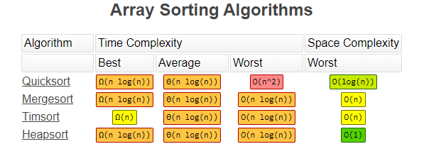
Heapsort has a typical time complexity of O(n log n). This is not a stable sorting algorithm however so there is no guarantee that items will be in their original order. This algorithm works by placing items on a binary tree where the root node is the maximum value. Then it will deconstruct that tree to form the sorted array.

Mergesort is a divide and conquer algorithm that has a typical time complexity of O(n log n). This algorithm separates the list in half and those halves in half until there are individual elements left. Then the elements are paired up, sorted, and merged repeatedly until the list is complete again. This algorithm is stable so it is great where that is necessary.

Quicksort is one very commonly used algorithm as it is easy to implement and has an average time complexity of O(n log n). The problem with this is everything is based around picking a good pivot point that is already in the proper place and sorting around it. Picking a poor pivot point could lead to an O(n²) time complexity. This tied with the fact that it is not stable leads me to not recommend it.

Timsort is a sort that you may not have ever heard of. This sort, named for its inventor Tim Peters, is a combination of a binary search, insert sort, and a merge sort. Its average time complexity is O(n log n) however it is able to hit this with better consistency and has a best-case complexity of O(n). Also, this is a stable algorithm which makes it great to use anywhere.

The best part is using Timsort in python only takes one line. That's right. It is the built-in sort function.array.sort()

Results: Timsort outperforms all the others which is why it is the core sorting algorithm for python. Next Mergesort and Quicksort are neck and neck. Finally, Heapsort is pulling up the rear… well, the rear of this list at least. There are plenty of worse sorting algorithms such as random sort.Algorithm:   Time:          
timsort      0.001594 ms
mergesort    0.033845 ms
quicksort    0.097097 ms
heapsort     0.365555 ms

Here is a chart that shows the Big O of all of these sorting algorithms. Also, we have space complexity which is how much extra space is needed to complete the algorithm.

That is all for this list. Now go forth and use these in your day to day Python and follow along for more tips and tricks.